This article is for beginners as well as intermediate level machine learning enthusiasts. Here, 10 most basic concepts are described in simple yet illustrative way.
1. Error, Mean Squared error, Irreducible and Reducible Error
Machine Learning model is generated based on algorithm it uses and training data it is given. A more aligned or uniform training data will yield simpler model, while a more varied and training data having outlier data will give complex model.
Performance of a Machine Learning model is judged based on prediction it makes. If we ask the model to predict output or dependent variable for a data which is already in training data, then we are more likely to close to accurate prediction.
True test of performance is done with a data different than training data. Therefore, it is always a best practice to split given data into 2 parts viz. training dataset and testing dataset. Performance or Prediction for testing dataset gives us clearer picture about Performance of model.
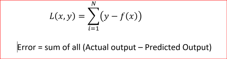
Let us say we have x as dependent or input variable and our model represented by function f to give y as independent or output variable. Prediction error for one test data will be difference between actual output and predicted output.
Similarly the Performance of the model is sum of all Prediction Error for test dataset.
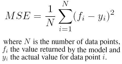
We take square of difference for each test data in order to avoid situation of negative error canceling out positive error. Minimizing Mean Squared Error is one of the way to achieve best performing model or function f.
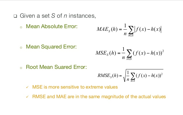
Other types of Error metrics:
Error is sum of reducible and irreducible error.
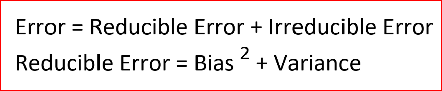
Irreducible Error: Errors which can't be removed no matter what algorithm you apply. These errors are caused by unknown variables that are affecting the independent/output variable but are not one of the dependent/input variable while designing the model.
Reducible Error: has two components - bias and variance. We will discuss in detail in following topic.
2. Bias and Variance and their trade-off
Bias Explaination
Unless the learned model predicts output of every test data accurately, there will always be difference between actual value and predicted value which is also called Error. Error is summation of differences of actual value and predicted value for each test data value.
We will absolute function for difference to not allow negative error balancing positive error.
Here is formula for Mean Absolute Error(MAE)
Bias Definition
Bias is basically the Mean Absolute Error. If summation of difference between actual value and predicted value is high, then Bias is high.
Low Bias means training data generates a model which quite accurately captures all training data and fits them well. Low Bias is also called a case of Overfitting, where model learns training data so well that it captured noises too.
High Bias means training data generates a model which misses the relevant relationship between input and output variable. It also means, that model is too simple and does not captures complexity of data distribution. High bias is also called case of Underfitting, where model did not learn training data well and could not capture underlying trend of data.
Variance Explaination
Variance: Once the model is generated using training data and model is given new data in form of test data or validation data. The ability of model to perform with new data is measured using Variance.
Variance Definition
Variance is measure of how scattered or out of sync the predicted value is with actual value.
High Variance denotes Overfitting caused because model is too flexible and captured random noises of training data as an important feature and responded to them. Such High Variances will yield out of sync or highly scattered data representation with new set of data input.
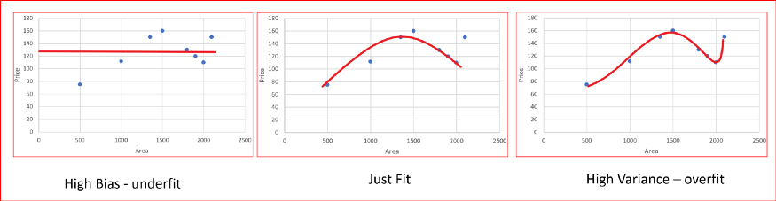
There is always a trade-off between Bias and Variance. Below figures explains it:
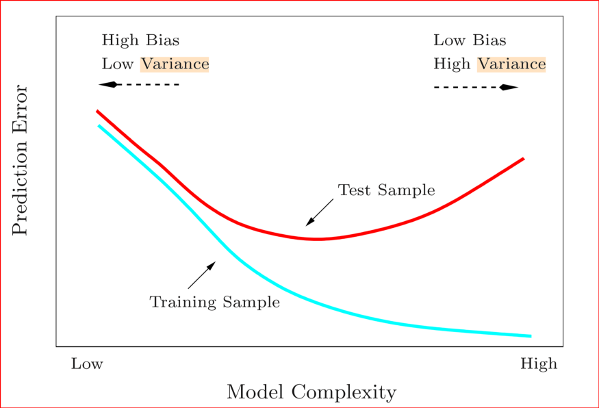
Performance of model will be good when there will be Low Bias and Low Variance.
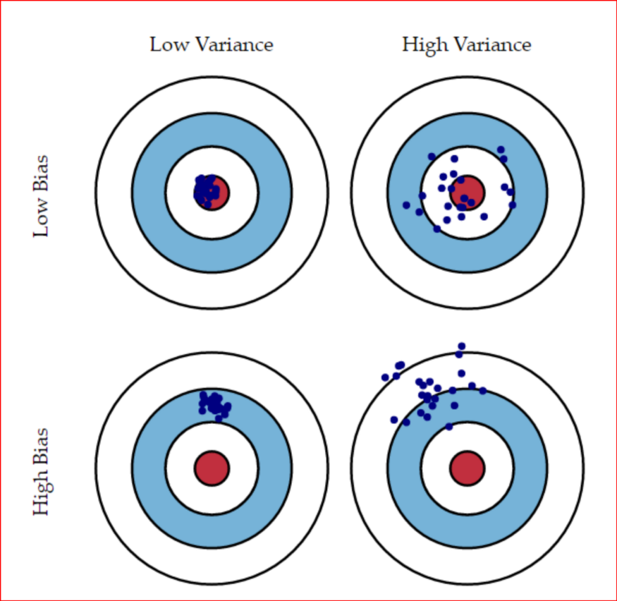
High Bias Low Variance: Models are consistent but inaccurate on average
High Bias High Variance : Models are inaccurate and also inconsistent on average
Low Bias Low Variance: Models are accurate and consistent on averages. We strive for this in our model
Low Bias High variance:Models are somewhat accurate but inconsistent on averages. A small change in the data can cause a large error.
3. Overfitting and Underfitting
Overfitting Definition
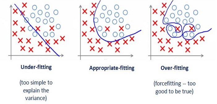
Overfitting: if noises of training data are captured in statistical model or machine learning model thereby making generated model quite complex, flexible and accommodating. Such cases are called Overfitting.
In simple language, if model represents training data too well, we say it to be overfit. For obvious reason, Overfit model will not perform good when given unseen or new data and asked to predict their output value.
Overfitting specifically occurs when Low Bias and High Variance.
Overfitting can be detected and avoided by fitting multiple models and using validation or cross-validation to compare their predictive accuracies on test data.
Underfitting Definition
Underfitting: if training data is not well represented by statistical model or machine learning model, thereby making generated model too simple to predict value for input data. Such cases are called Underfitting.
Underfitting specifically occurs when High Bias and Low Variance.
Both Overfitting and Underfitting are like cancer to Machine learning model. Both makes a model inefficient and inaccurate for new test data.
4. Cross Validation
One major task in Machine learning study is deciding which Machine learning algorithm will suit a particular set of problem. Some problem can be better addressed with Linear Regression, other with Logistic Regression, or K-Nearest Neighbours or Support Vector Machines. Now the question is, how we can compare the performance of different algorithm for a particular problem set.
Cross Validation allows us to compare different machine learning algorithm and helps us do comparative analysis among them.
Reusing the same dataset for training and then testing is terrible approach, as it will lead to model overfit and performance evaluation will capture wrong result. Hence we already know that, for given data set(collection of data). It is always best practice to split given dataset into training dataset and testing dataset.
Training dataset is used to generate a model while testing dataset is used for validating the model and produce it's performance. Let us say, we split dataset into 2 sets of 75%(training dataset) and 25%(testing dataset).
But, how we can compare different Algorithm based on same split. And how we can be sure that which split will be best like choosing first 75% as training and last 25% as test data, or first 25% as test and rest 75% as training data?
The answer is Cross Validation!
There are 2 approaches under Cross Validation.
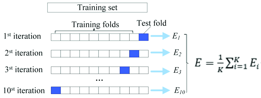
- K-fold Cross Validation: Split the dataset into k numbers of subset, then we perform training on (k-1) subsets and testing on 1 subset. We keep iterating such that, each subset will get chance as testing subset. Basically, k iteration happens.
- Leave One Out Cross Validation(LOOCV): It can be interpreted as K-fold Cross validation, where K is number of data items in dataset. So, basically here we train model using (n - 1) data items and leave just 1 data for testing. This process is repeated for each data item to be choosen as testing once. Hence, n iteration takes place.
Advantages/Disadvantages of K-Fold Cross Validation
- Faster. Selection of K is important. Ideally K = 10 for large dataset is found good.
Advantages/Disadvantages of LOOCV
- Easy to understand.
- Leads to higher variation, as only one data item is left for testing. An outlier data item in dataset will lead to higher variance.
- Takes more time.
5. Confusion Matrix
With a problem set where we need to apply machine learning algorithm to find which algorithm suits the situation best. We divide dataset into two parts namely training dataset and testing/validating dataset.
Once a model is generated with training dataset, we test/evaluate it using Confusion Matrix.
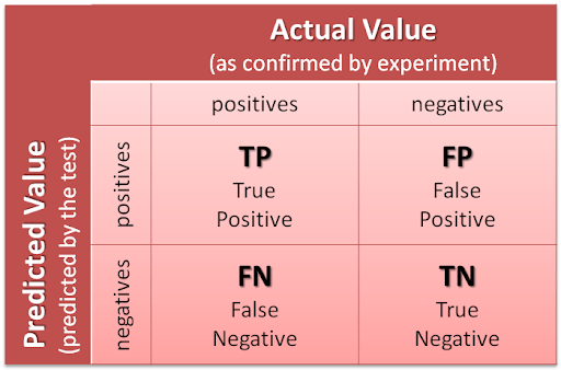
Confusion or Error Matrix is a matrix or table representation for performance of a classification model on test dataset for which actual value is known. In the Confusion matrix rows and columns are constituted by number of classes and each possible pairs are for Predicted and Actual classes have their value.
Remember, Rows corresponds to what was predicted, while columns corresponds to Actual or True value.
For example for two classes case:
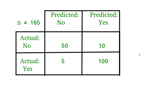
Example for dataset containing n = 165 data items.
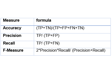
Various parameter are further used to evaluate the model:
Thank you for reading it all along. Hope you liked this article!!
About the author